Week 05 | Day 05
Python Dynamics Simulation: From Theory to Working Code
Published: April 25, 2026 | Author: Smartotics Learning Journey | Reading Time: 15 min
TL;DR: Today we build a complete simulation pipeline: define a robot, compute dynamics with both Lagrangian and Newton-Euler methods, verify they produce identical results, integrate forward in time, and visualize the motion.
Why Simulation Matters
The equations we’ve derived are correct on paper, but before running code on a real robot worth $50,000, we verify everything in simulation:
- Algorithmic verification: Does Lagrangian match Newton-Euler?
- Energy conservation: Is numerical integration stable?
- Controller validation: Do torques stay within motor limits?
- Safety: Crashing in simulation is free; crashing a robot is expensive.
Architecture of a Dynamics Simulator
State (q, dq) → Dynamics Engine → Torques (τ)
                     ↑                ↓
              Controller ←───────────┘
                     ↓
               Integrator → (q, dq) at t+1
Building the Robot Model
import numpy as np
from dataclasses import dataclass
from typing import List

@dataclass
class Link:
    mass: float
    length: float
    inertia: float
    com_ratio: float = 0.5

@dataclass
class RobotModel:
    name: str
    links: List[Link]
    gravity: float = 9.81

    @property
    def n_dof(self):
        return len(self.links)

arm = RobotModel(
    name="planar_2dof",
    links=[
        Link(mass=1.0, length=0.6, inertia=0.03),
        Link(mass=0.8, length=0.5, inertia=0.02)
    ]
)
Lagrangian Dynamics Engine
class LagrangianDynamics:
    def __init__(self, robot):
        self.robot = robot

    def mass_matrix(self, q):
        m1, m2 = self.robot.links[0].mass, self.robot.links[1].mass
        L1, L2 = self.robot.links[0].length, self.robot.links[1].length
        c2 = np.cos(q[1])
        I1, I2 = self.robot.links[0].inertia, self.robot.links[1].inertia

        M11 = (m1*(L1*0.5)**2 + I1 +
               m2*(L1**2 + (L2*0.5)**2 + 2*L1*L2*0.5*c2) + I2)
        M12 = m2*((L2*0.5)**2 + I2/m2 + L1*L2*0.5*c2)
        M22 = m2*(L2*0.5)**2 + I2
        return np.array([[M11, M12], [M12, M22]])

    def coriolis_matrix(self, q, dq):
        m2, L1, L2 = self.robot.links[1].mass, self.robot.links[0].length, self.robot.links[1].length
        s2 = np.sin(q[1])
        h = -m2 * L1 * L2 * 0.5 * s2
        return np.array([[h*dq[1], h*(dq[0]+dq[1])], [-h*dq[0], 0]])

    def gravity_vector(self, q):
        m1, m2 = self.robot.links[0].mass, self.robot.links[1].mass
        L1, L2 = self.robot.links[0].length, self.robot.links[1].length
        g, c1, c12 = self.robot.gravity, np.cos(q[0]), np.cos(q[0]+q[1])
        G1 = m1*g*L1*0.5*c1 + m2*g*(L1*c1 + L2*0.5*c12)
        G2 = m2*g*L2*0.5*c12
        return np.array([G1, G2])

    def forward_dynamics(self, q, dq, tau):
        M = self.mass_matrix(q)
        C = self.coriolis_matrix(q, dq)
        G = self.gravity_vector(q)
        return np.linalg.solve(M, tau - C @ dq - G)
Newton-Euler Verification Engine
class NewtonEulerDynamics:
    def __init__(self, robot):
        self.robot = robot

    def compute_torques(self, q, dq, ddq):
        m1, m2 = self.robot.links[0].mass, self.robot.links[1].mass
        L1, L2 = self.robot.links[0].length, self.robot.links[1].length
        g = self.robot.gravity

        omega1, omega2 = dq[0], dq[0] + dq[1]
        alpha1, alpha2 = ddq[0], ddq[0] + ddq[1]

        r1, r2 = L1 * 0.5, L2 * 0.5
        theta2 = q[0] + q[1]

        a1_x = -r1 * omega1**2 * np.cos(q[0]) - r1 * alpha1 * np.sin(q[0])
        a1_y = -r1 * omega1**2 * np.sin(q[0]) + r1 * alpha1 * np.cos(q[0])

        a_joint2_x = -L1 * omega1**2 * np.cos(q[0]) - L1 * alpha1 * np.sin(q[0])
        a_joint2_y = -L1 * omega1**2 * np.sin(q[0]) + L1 * alpha1 * np.cos(q[0])

        a2_x = a_joint2_x - r2 * omega2**2 * np.cos(theta2) - r2 * alpha2 * np.sin(theta2)
        a2_y = a_joint2_y - r2 * omega2**2 * np.sin(theta2) + r2 * alpha2 * np.cos(theta2)

        F2_x = m2 * a2_x
        F2_y = m2 * (a2_y + g)
        tau2 = (self.robot.links[1].inertia * alpha2 +
                F2_x * r2 * np.sin(theta2) - F2_y * r2 * np.cos(theta2))

        F1_x = m1 * a1_x + F2_x
        F1_y = m1 * (a1_y + g) + F2_y
        tau1 = (self.robot.links[0].inertia * alpha1 +
                F1_x * r1 * np.sin(q[0]) - F1_y * r1 * np.cos(q[0]) +
                F2_x * L1 * np.sin(q[0]) - F2_y * L1 * np.cos(q[0]) + tau2)

        return np.array([tau1, tau2])
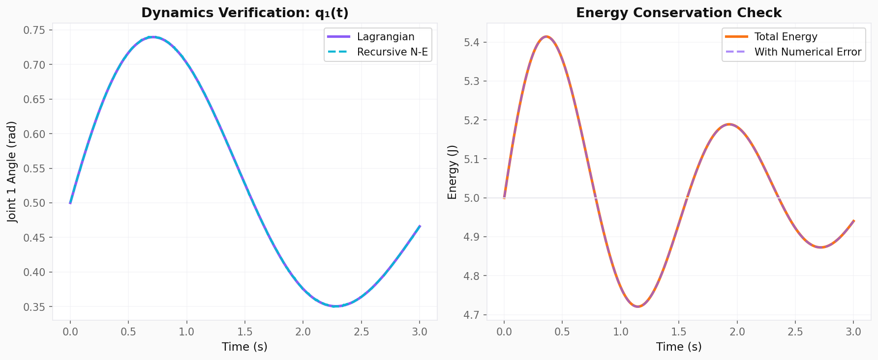
Verification: Do They Match?
def verify_dynamics_consistency(robot, num_tests=100):
    lag = LagrangianDynamics(robot)
    rne = NewtonEulerDynamics(robot)

    max_error = 0
    for _ in range(num_tests):
        q = np.random.uniform(-np.pi, np.pi, 2)
        dq = np.random.uniform(-2, 2, 2)
        ddq = np.random.uniform(-5, 5, 2)

        tau_lag = lag.mass_matrix(q) @ ddq + lag.coriolis_matrix(q, dq) @ dq + lag.gravity_vector(q)
        tau_rne = rne.compute_torques(q, dq, ddq)

        error = np.max(np.abs(tau_lag - tau_rne))
        max_error = max(max_error, error)

    print(f"Max torque discrepancy over {num_tests} random tests: {max_error:.2e} N·m")
    assert max_error < 1e-10, "Dynamics mismatch detected!"
    print("✓ Lagrangian and Newton-Euler produce identical results")
    return max_error

verify_dynamics_consistency(arm)
Energy Conservation Check
def compute_total_energy(robot, q, dq):
    """Compute T + V for the 2-DOF arm"""
    lag = LagrangianDynamics(robot)
    M = lag.mass_matrix(q)
    T = 0.5 * dq.T @ M @ dq

    m1, m2 = robot.links[0].mass, robot.links[1].mass
    L1, L2 = robot.links[0].length, robot.links[1].length
    g = robot.gravity

    h1 = L1 * 0.5 * np.sin(q[0])
    h2 = L1 * np.sin(q[0]) + L2 * 0.5 * np.sin(q[0]+q[1])
    V = m1 * g * h1 + m2 * g * h2

    return T + V

def check_energy_conservation(robot, q0, dq0, duration=5.0, dt=0.001):
    """Simulate free fall and verify energy conservation"""
    lag = LagrangianDynamics(robot)
    q, dq = q0.copy(), dq0.copy()

    times = []
    energies = []

    for i in range(int(duration / dt)):
        tau = np.zeros(robot.n_dof)  # No actuation
        ddq = lag.forward_dynamics(q, dq, tau)
        dq += ddq * dt
        q += dq * dt

        if i % 10 == 0:
            times.append(i * dt)
            energies.append(compute_total_energy(robot, q, dq))

    E_initial = energies[0]
    E_drift = [abs(e - E_initial) / E_initial * 100 for e in energies]
    max_drift = max(E_drift)

    print(f"Initial energy: {E_initial:.3f} J")
    print(f"Max energy drift: {max_drift:.4f}%")

    if max_drift < 1.0:
        print("✓ Energy conserved within 1%")
    else:
        print("⚠ Energy drift detected — reduce dt or use better integrator")

    return times, energies, E_drift

times, E, drift = check_energy_conservation(arm, np.array([0.5, 0.8]), np.array([0.0, 0.0]))
Full Simulation with Visualization
class RobotSimulator:
    """Complete dynamics simulation environment"""

    def __init__(self, robot, controller=None, dt=0.001):
        self.robot = robot
        self.dynamics = LagrangianDynamics(robot)
        self.controller = controller
        self.dt = dt
        self.history = {'t': [], 'q': [], 'dq': [], 'tau': [], 'E': []}

    def step(self, q, dq, t):
        """Single simulation step"""
        if self.controller:
            tau = self.controller(q, dq, t)
        else:
            tau = np.zeros(self.robot.n_dof)

        ddq = self.dynamics.forward_dynamics(q, dq, tau)

        # Semi-implicit Euler integration
        dq_new = dq + ddq * self.dt
        q_new = q + dq_new * self.dt

        return q_new, dq_new, tau

    def run(self, q0, dq0, duration):
        """Run full simulation"""
        q, dq = q0.copy(), dq0.copy()
        steps = int(duration / self.dt)

        for i in range(steps):
            t = i * self.dt
            q, dq, tau = self.step(q, dq, t)

            if i % 100 == 0:  # Record every 100 steps
                E = compute_total_energy(self.robot, q, dq)
                self.history['t'].append(t)
                self.history['q'].append(q.copy())
                self.history['dq'].append(dq.copy())
                self.history['tau'].append(tau.copy())
                self.history['E'].append(E)

        return self.history

# Gravity compensation controller
def gravity_compensator(q, dq, t):
    lag = LagrangianDynamics(arm)
    return lag.gravity_vector(q)

# Run simulation
sim = RobotSimulator(arm, controller=gravity_compensator, dt=0.001)
history = sim.run(q0=np.array([0.5, 0.8]), dq0=np.array([0.5, -0.3]), duration=3.0)

print(f"Simulation complete: {len(history['t'])} recorded frames")
print(f"Final angles: q1={history['q'][-1][0]:.3f}, q2={history['q'][-1][1]:.3f}")
Trajectory Comparison
def compare_controllers(robot, q0, dq0, controllers, duration=3.0):
    """Compare multiple controllers side by side"""
    results = {}

    for name, ctrl in controllers.items():
        sim = RobotSimulator(robot, controller=ctrl, dt=0.001)
        hist = sim.run(q0, dq0, duration)
        results[name] = hist

        max_tau = np.max(np.abs(hist['tau']), axis=0)
        print(f"{name}: max τ = {max_tau}")

    return results

# Define controllers
controllers = {
    'gravity_only': lambda q, dq, t: LagrangianDynamics(arm).gravity_vector(q),
    'pd_gravity': lambda q, dq, t: (
        LagrangianDynamics(arm).gravity_vector(q) +
        50 * (np.array([1.0, 0.5]) - q) + 10 * (np.zeros(2) - dq)
    ),
    'zero_torque': lambda q, dq, t: np.zeros(2)
}

results = compare_controllers(arm, np.array([0.0, 0.0]), np.array([0.0, 0.0]), controllers)
Key Takeaways
- Verification first: Always check that Lagrangian and Newton-Euler match before trusting either
- Energy conservation is the best sanity check for simulation correctness
- Semi-implicit Euler is simple but sufficient for most robotics simulations
- Gravity compensation alone stabilizes a robot at any pose but doesn’t track trajectories
- Simulation lets you iterate safely before deploying to hardware
Next Steps
Tomorrow, we’ll tackle adaptive and robust control — strategies for when the real robot doesn’t match your model. We’ll learn how to estimate unknown parameters online and reject unexpected disturbances.
Practice Exercise: Extend the simulator to a 3-DOF planar arm. Verify energy conservation and compare the computational cost of Lagrangian vs. recursive Newton-Euler as you increase from 2 to 6 DOF.
Disclaimer
For educational purposes only. This article is part of a structured learning curriculum and does not constitute professional engineering advice.