Week 05 | Day 01

Robot Dynamics Fundamentals: Mass, Inertia, and Forces

Published: April 20, 2026 | Author: Smartotics Learning Journey | Reading Time: 12 min

TL;DR: Dynamics answers the question: “Given forces and torques applied to a robot, how does it move?” We cover mass properties, inertia tensors, Newton-Euler equations for rigid bodies, and set up the mathematical foundation for the entire week.

---

Why Dynamics Matters

So far, we’ve mastered kinematics — the geometry of motion. We can compute where a robot’s end-effector is (forward kinematics) and what joint angles achieve a desired pose (inverse kinematics). We can also plan collision-free paths.

But kinematics is only half the story. It tells us where the robot should go, not how to get there given real-world constraints:

• Motors have torque limits
• Links have mass that resists acceleration
• External forces (gravity, collisions) affect motion
• Energy consumption depends on how we move

Dynamics bridges the gap between desired motion and the forces required to achieve it.

---

The Big Picture: Dynamics vs. Kinematics

Aspect	Kinematics	Dynamics
Input	Joint positions/velocities	Forces and torques
Output	Position, velocity, acceleration	Required forces for desired motion
Question	”Where is the end-effector?"	"What torque do I need to move there?”
Key concepts	D-H parameters, Jacobians	Mass, inertia, equations of motion

---

Mass Properties of Robots

Every link in a robot has three critical mass properties:

1. Mass (m)

The total mass of the link. Simple, but crucial for gravitational loading and inertial resistance.

2. Center of Mass (COM)

The point where the link’s mass is concentrated. For a uniform rod of length L, the COM is at L/2. For complex shapes, we compute:

r_com = (∫ r dm) / m

3. Inertia Tensor (I)

The rotational analog of mass. It describes how mass is distributed relative to the COM and determines resistance to angular acceleration.

For a 3D rigid body, the inertia tensor is a 3×3 symmetric matrix:

I = [ Ixx  -Ixy  -Ixz ]
    [ -Ixy  Iyy  -Iyz ]
    [ -Ixz  -Iyz  Izz ]

Where:

• Ixx = ∫(y² + z²) dm (resistance to rotation about x-axis)
• Ixy = ∫(xy) dm (product of inertia)

Common Shape Inertias

Shape	I (about COM)
Thin rod (mass m, length L)	I = (1/12)mL²
Solid cylinder (mass m, radius R)	I = (1/2)mR²
Solid sphere (mass m, radius R)	I = (2/5)mR²
Rectangular plate (m, a×b)	I = (1/12)m(a² + b²)

---

Newton-Euler for a Single Rigid Body

For a single rigid body, the equations of motion are:

Linear motion (Newton’s Second Law):

F = m · a_com

Angular motion (Euler’s Equation):

τ = I · α + ω × (I · ω)

Where:

• F: Total external force
• τ: Total external torque
• a_com: Linear acceleration of COM
• α: Angular acceleration
• ω: Angular velocity
• The ω × (I · ω) term is the gyroscopic torque — it appears when the body rotates about multiple axes simultaneously.

---

Forces Acting on Robot Links

Each robot link experiences several forces:

1. Gravity: F_g = m · g (acts at COM, downward)
2. Joint torques: τ_i (actuated forces from motors)
3. Constraint forces: Forces transmitted through joints from adjacent links
4. External forces: Contact forces, payloads, disturbances

Free Body Diagram Approach

To analyze a robot link, we isolate it and identify all forces:

import numpy as np

class RigidBodyDynamics:
    """Dynamics of a single rigid body in 3D space"""
    
    def __init__(self, mass, inertia_tensor, com_position):
        self.m = mass
        self.I = np.array(inertia_tensor)  # 3x3 inertia tensor
        self.r_com = np.array(com_position)
        
        # State variables
        self.position = np.zeros(3)
        self.velocity = np.zeros(3)
        self.acceleration = np.zeros(3)
        self.orientation = np.eye(3)  # Rotation matrix
        self.omega = np.zeros(3)      # Angular velocity
        self.alpha = np.zeros(3)      # Angular acceleration
    
    def compute_linear_dynamics(self, external_forces):
        """
        Calculate linear acceleration from external forces
        
        Args:
            external_forces: Total external force vector [Fx, Fy, Fz]
        
        Returns:
            Linear acceleration
        """
        F_total = np.array(external_forces)
        a = F_total / self.m
        return a
    
    def compute_angular_dynamics(self, external_torques):
        """
        Calculate angular acceleration from external torques
        
        Args:
            external_torques: Total external torque vector [τx, τy, τz]
        
        Returns:
            Angular acceleration
        """
        tau = np.array(external_torques)
        
        # Euler equation: τ = I·α + ω×(I·ω)
        I_omega = self.I @ self.omega
        gyroscopic = np.cross(self.omega, I_omega)
        
        # Solve for angular acceleration
        alpha = np.linalg.solve(self.I, tau - gyroscopic)
        return alpha
    
    def update_state(self, force, torque, dt):
        """
        Update body state given force and torque over time step dt
        
        Args:
            force: External force [Fx, Fy, Fz]
            torque: External torque [τx, τy, τz]
            dt: Time step
        """
        # Compute accelerations
        self.acceleration = self.compute_linear_dynamics(force)
        self.alpha = self.compute_angular_dynamics(torque)
        
        # Integrate (simple Euler integration)
        self.velocity += self.acceleration * dt
        self.position += self.velocity * dt
        self.omega += self.alpha * dt
        
        return {
            'position': self.position,
            'velocity': self.velocity,
            'acceleration': self.acceleration,
            'omega': self.omega,
            'alpha': self.alpha
        }

# Example: Simple pendulum dynamics
pendulum = RigidBodyDynamics(
    mass=2.0,
    inertia_tensor=[[0, 0, 0], [0, 0, 0], [0, 0, 0.5]],  # Rotate about z
    com_position=[0, 0.5, 0]
)

# Gravity force
gravity = [0, -2.0 * 9.81, 0]
# No external torque (pivot provides constraint torque)
torque = [0, 0, 0]

state = pendulum.update_state(gravity, torque, dt=0.01)
print(f"Acceleration: {state['acceleration']}")
print(f"Angular acceleration: {state['alpha']}")

---

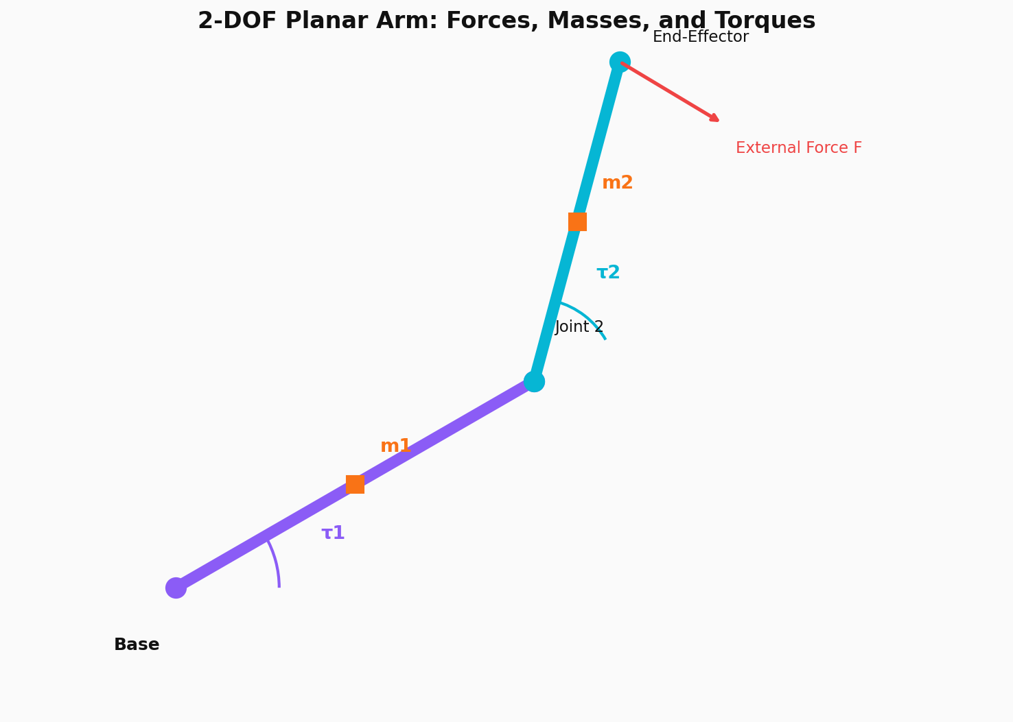
2D Planar Arm Dynamics

Let’s derive the dynamics for a 2-DOF planar arm — the simplest non-trivial robot.

Lagrangian Setup (Preview)

For a 2-link planar arm with masses m₁, m₂ and lengths L₁, L₂:

Kinetic Energy:

T = ½(m₁v₁² + m₂v₂²) + ½(I₁ω₁² + I₂ω₂²)

Potential Energy:

V = m₁gh₁ + m₂gh₂

Where h₁ and h₂ are the vertical heights of each link’s COM.

The equations of motion take the standard form:

τ = M(q)·q̈ + C(q, q̇)·q̇ + G(q)

Where:

• M(q): Mass matrix (inertia, depends on configuration)
• C(q, q̇): Coriolis and centrifugal terms
• G(q): Gravity terms
• τ: Joint torques

Mass Matrix Intuition

The mass matrix M(q) tells us how much torque is needed to accelerate each joint, considering the entire robot configuration:

def compute_2dof_mass_matrix(q1, q2, m1, m2, L1, L2):
    """
    Compute mass matrix for 2-DOF planar arm
    
    Args:
        q1, q2: Joint angles (rad)
        m1, m2: Link masses (kg)
        L1, L2: Link lengths (m)
    
    Returns:
        2x2 mass matrix M(q)
    """
    c2 = np.cos(q2)
    
    M11 = m1*L1**2/3 + m2*(L1**2 + L1*L2*c2 + L2**2/3)
    M12 = m2*(L1*L2*c2/2 + L2**2/3)
    M21 = M12  # Symmetric
    M22 = m2*L2**2/3
    
    return np.array([[M11, M12], [M21, M22]])

# Example
M = compute_2dof_mass_matrix(q1=0.5, q2=1.0, m1=1.0, m2=0.8, L1=0.6, L2=0.5)
print("Mass matrix M(q):")
print(M)
print(f"Effective inertia at joint 1: {M[0,0]:.3f} kg·m²")

Key insight: The mass matrix changes with joint angles. When the elbow is fully extended (q₂ = 0), joint 1 feels the full inertia of both links. When folded (q₂ = π), the effective inertia is minimized.

---

Gravity Loading

Gravity creates torques at each joint that motors must counteract:

def compute_gravity_torques(q1, q2, m1, m2, L1, L2, g=9.81):
    """
    Compute gravity torques for 2-DOF planar arm
    
    Args:
        q1, q2: Joint angles
        m1, m2: Link masses
        L1, L2: Link lengths
        g: Gravity acceleration
    
    Returns:
        [τ1_gravity, τ2_gravity]
    """
    c1, s1 = np.cos(q1), np.sin(q1)
    c12, s12 = np.cos(q1+q2), np.sin(q1+q2)
    
    # Gravity torque at joint 2
    tau2 = m2 * g * (L2/2) * c12
    
    # Gravity torque at joint 1
    tau1 = m1 * g * (L1/2) * c1 + m2 * g * (L1 * c1 + (L2/2) * c12)
    
    return np.array([tau1, tau2])

# Example: gravity torques at different configurations
configs = [
    ('Arm down', [0, 0]),
    ('Arm horizontal', [np.pi/2, 0]),
    ('Arm up', [np.pi, 0]),
]

for name, (q1, q2) in configs:
    tau_g = compute_gravity_torques(q1, q2, m1=1.0, m2=0.8, L1=0.6, L2=0.5)
    print(f"{name}: τ₁ = {tau_g[0]:.2f} N·m, τ₂ = {tau_g[1]:.2f} N·m")

---

Key Takeaways

• Dynamics extends kinematics by relating forces to motion, essential for real robot control
• Mass matrix M(q) captures how configuration affects inertial loading at each joint
• Gravity torques G(q) must be compensated by motors and vary with robot pose
• Coriolis/centrifugal terms C(q, q̇) become significant at high speeds
• The standard dynamics form τ = M(q)·q̈ + C(q, q̇)·q̇ + G(q) is the foundation for all advanced control

---

Next Steps

Tomorrow, we’ll derive these equations systematically using the Lagrangian method — a powerful energy-based approach that avoids force-balance bookkeeping and scales elegantly to complex robots.

Practice Exercise: Compute the mass matrix and gravity torques for a 3-DOF planar arm. How does the mass matrix change when you add a third link? Plot M₁₁(q₂, q₃) as a heatmap to visualize configuration-dependent inertia.

---

Disclaimer

For educational purposes only. This article is part of a structured learning curriculum and does not constitute professional engineering advice.