Week 05 | Day 06
Adaptive and Robust Control: Handling Uncertainty
Published: April 26, 2026 | Author: Smartotics Learning Journey | Reading Time: 14 min
TL;DR: Real robots never match their models exactly. Adaptive control estimates unknown parameters online. Robust control guarantees performance despite bounded uncertainty. Together, they make robots reliable in the real world.
The Reality Gap
Every controller we’ve built so far assumes we know the robot’s dynamics perfectly. In reality:
- Payloads change (a robot picks up different objects)
- Friction varies with temperature and wear
- Links flex slightly under load
- Gear backlash introduces dead zones
- External disturbances push the robot unexpectedly
The model is always wrong. The question is: can we control anyway?
Two Philosophies
| Approach | Strategy | When to Use |
|---|---|---|
| Adaptive | Learn parameters online | Slow changes, structured uncertainty (unknown mass, inertia) |
| Robust | Design for worst case | Fast disturbances, unstructured uncertainty (friction, backlash) |
These aren’t mutually exclusive — the best systems often combine both.
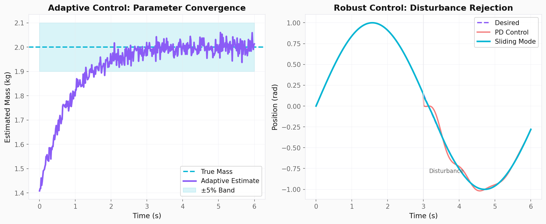
Adaptive Control: Online Parameter Estimation
The Core Idea
Instead of using fixed model parameters, estimate them while the robot moves. Update the estimates based on the prediction error between expected and actual motion.
Adaptive Controller for a 2-DOF Arm
import numpy as np

class AdaptiveController:
    """
    Adaptive inverse dynamics controller with online mass estimation

    Estimates unknown payload mass and updates control law in real-time.
    """

    def __init__(self, robot, gamma=0.5, lambda_reg=0.01):
        """
        Args:
            robot: RobotModel with known structure but uncertain parameters
            gamma: Adaptation gain (learning rate)
            lambda_reg: Regularization to prevent parameter drift
        """
        self.robot = robot
        self.n_dof = robot.n_dof

        # Adaptation gain
        self.gamma = gamma
        self.lambda_reg = lambda_reg

        # Parameter estimates (start with initial guesses)
        self.m2_hat = robot.links[1].mass  # Estimate of link 2 mass
        self.m2_true = robot.links[1].mass

        # Tracking error integral (for anti-drift)
        self.error_integral = np.zeros(self.n_dof)

    def compute_regressor(self, q, dq, ddq):
        """
        Compute the regressor matrix Y(q, dq, ddq) such that:
        τ = Y(q, dq, ddq) · θ

        For a 2-DOF arm, θ = [m1, m2] (masses to estimate)
        """
        L1, L2 = self.robot.links[0].length, self.robot.links[1].length
        g = self.robot.gravity
        c1, c2, c12 = np.cos(q[0]), np.cos(q[1]), np.cos(q[0]+q[1])
        s2 = np.sin(q[1])

        # Simplified regressor for mass estimation
        # Y[i,j] = contribution of parameter j to torque i
        Y = np.zeros((self.n_dof, 2))

        # m1 contributions
        Y[0, 0] = (L1**2/3) * ddq[0] + g * L1 * 0.5 * c1
        Y[1, 0] = 0

        # m2 contributions
        Y[0, 1] = ((L1**2 + (L2*0.5)**2 + L1*L2*c2) * ddq[0] +
                   (L1*L2*0.5*c2 + (L2*0.5)**2) * ddq[1] -
                   L1*L2*0.5*s2 * (dq[1]**2 + 2*dq[0]*dq[1]) +
                   g * (L1*c1 + L2*0.5*c12))
        Y[1, 1] = ((L1*L2*0.5*c2 + (L2*0.5)**2) * ddq[0] +
                   (L2*0.5)**2 * ddq[1] +
                   L1*L2*0.5*s2 * dq[0]**2 +
                   g * L2*0.5*c12)

        return Y

    def control(self, q, dq, q_desired, dq_desired, ddq_desired, dt):
        """
        Compute adaptive control torque

        τ = Y(q, dq, ddq_desired) · θ̂ + Kv · s
        where s = (dq_desired - dq) + Λ(q_desired - q)
        """
        # Tracking errors
        q_err = q_desired - q
        dq_err = dq_desired - dq

        # Sliding surface
        Lambda = np.diag([5.0, 5.0])
        s = dq_err + Lambda @ q_err

        # Reference acceleration
        ddq_ref = ddq_desired + Lambda @ dq_err

        # Regressor with reference acceleration
        Y = self.compute_regressor(q, dq, ddq_ref)

        # Parameter vector estimate
        theta_hat = np.array([self.robot.links[0].mass, self.m2_hat])

        # Control law
        Kv = np.diag([20.0, 10.0])
        tau = Y @ theta_hat + Kv @ s

        # Parameter update (gradient descent on prediction error)
        # θ̇ = -Γ · Yᵀ · s
        dtheta = -self.gamma * Y.T @ s - self.lambda_reg * (theta_hat - np.array([self.robot.links[0].mass, self.m2_hat]))
        self.m2_hat += dtheta[1] * dt

        # Keep estimate positive and bounded
        self.m2_hat = np.clip(self.m2_hat, 0.1, 5.0)

        return tau, self.m2_hat

# Test: robot picks up unknown payload
arm = RobotModel(
    name="planar_2dof",
    links=[Link(mass=1.0, length=0.6, inertia=0.03),
           Link(mass=0.8, length=0.5, inertia=0.02)]
)

ctrl = AdaptiveController(arm, gamma=1.0)

# Simulate payload change at t=2s
q, dq = np.array([0.5, 0.5]), np.array([0.0, 0.0])
history = {'t': [], 'm2_hat': [], 'q_err': []}

for i in range(5000):
    t = i * 0.001

    # Payload increases at t=2
    if t > 2.0:
        arm.links[1].mass = 1.5  # True mass changes

    q_des = np.array([0.8, 0.3])
    dq_des = np.zeros(2)
    ddq_des = np.zeros(2)

    tau, m2_est = ctrl.control(q, dq, q_des, dq_des, ddq_des, dt=0.001)

    # Simulate robot motion
    lag = LagrangianDynamics(arm)
    ddq = lag.forward_dynamics(q, dq, tau)
    dq += ddq * 0.001
    q += dq * 0.001

    if i % 100 == 0:
        history['t'].append(t)
        history['m2_hat'].append(m2_est)
        history['q_err'].append(np.linalg.norm(q_des - q))

print(f"Final mass estimate: {history['m2_hat'][-1]:.3f} kg (true: {arm.links[1].mass} kg)")
Robust Control: Sliding Mode Control
The Core Idea
Define a “sliding surface” in state space. Drive the system onto this surface and keep it there, regardless of disturbances. The controller is intentionally discontinuous — it switches rapidly to counteract uncertainty.
Sliding Mode Controller
class SlidingModeController:
    """
    Sliding Mode Control (SMC) for robot manipulators

    Guarantees convergence despite bounded model uncertainty.
    """

    def __init__(self, robot, Lambda, K_slide, eta):
        """
        Args:
            robot: Nominal robot model
            Lambda: Sliding surface gain matrix
            K_slide: Switching gain (must exceed max uncertainty)
            eta: Boundary layer thickness (reduces chattering)
        """
        self.robot = robot
        self.Lambda = np.diag(Lambda)
        self.K_slide = np.diag(K_slide)
        self.eta = eta

        # Nominal dynamics
        self.dynamics = LagrangianDynamics(robot)

    def nominal_dynamics(self, q, dq, ddq):
        """Compute nominal torques using known model"""
        M = self.dynamics.mass_matrix(q)
        C = self.dynamics.coriolis_matrix(q, dq)
        G = self.dynamics.gravity_vector(q)
        return M @ ddq + C @ dq + G

    def control(self, q, dq, q_desired, dq_desired, ddq_desired):
        """
        Compute sliding mode control torque

        τ = M·q̈_ref + C·q̇ + G - K·sat(s/η)
        """
        # Tracking errors
        q_err = q_desired - q
        dq_err = dq_desired - dq

        # Sliding surface: s = dq_err + Λ·q_err
        s = dq_err + self.Lambda @ q_err

        # Reference acceleration
        ddq_ref = ddq_desired + self.Lambda @ dq_err

        # Nominal dynamics
        tau_nominal = self.nominal_dynamics(q, dq, ddq_ref)

        # Sliding term with saturation (reduces chattering)
        # sat(s/η) = s/η if |s/η| < 1, else sign(s)
        sat = np.clip(s / self.eta, -1, 1)
        tau_slide = -self.K_slide @ sat

        return tau_nominal + tau_slide, s

# Example: SMC with 30% model uncertainty
smc = SlidingModeController(
    robot=arm,
    Lambda=[5.0, 5.0],
    K_slide=[50.0, 30.0],  # Must exceed max disturbance
    eta=0.1                # Boundary layer
)

# Simulate with external disturbance
q, dq = np.array([0.0, 0.0]), np.array([0.0, 0.0])
disturbance = np.array([5.0, 3.0])  # N·m external push

for i in range(3000):
    t = i * 0.001
    q_des = np.array([1.0, 0.5])
    dq_des = np.zeros(2)
    ddq_des = np.zeros(2)

    tau, s = smc.control(q, dq, q_des, dq_des, ddq_des)
    tau += disturbance * (1 if t > 1.5 else 0)  # Disturbance at t=1.5

    lag = LagrangianDynamics(arm)
    ddq = lag.forward_dynamics(q, dq, tau)
    dq += ddq * 0.001
    q += dq * 0.001

print(f"Final error: {np.linalg.norm(q_des - q):.4f} rad")
print(f"Sliding surface: s = [{s[0]:.3f}, {s[1]:.3f}]")
Comparison: PD vs. Adaptive vs. Robust
def benchmark_controllers(robot, scenario, duration=5.0):
    """
    Compare PD, Adaptive, and Sliding Mode controllers
    """
    controllers = {
        'PD': lambda q, dq, t: (
            100 * (scenario['q_des'] - q) + 20 * (-dq)
        ),
        'Adaptive': AdaptiveController(robot, gamma=1.0).control,
        'Sliding Mode': SlidingModeController(
            robot, Lambda=[5,5], K_slide=[50,30], eta=0.1
        ).control
    }

    results = {}
    for name, ctrl in controllers.items():
        q, dq = scenario['q0'].copy(), scenario['dq0'].copy()
        errors = []
        torques = []

        for i in range(int(duration / 0.001)):
            t = i * 0.001

            if name == 'Adaptive':
                tau, _ = ctrl(q, dq, scenario['q_des'], np.zeros(2), np.zeros(2), 0.001)
            elif name == 'Sliding Mode':
                tau, _ = ctrl(q, dq, scenario['q_des'], np.zeros(2), np.zeros(2))
            else:
                tau = ctrl(q, dq, t)

            # Apply disturbance
            if t > scenario.get('disturbance_time', 999):
                tau += scenario['disturbance']

            lag = LagrangianDynamics(robot)
            ddq = lag.forward_dynamics(q, dq, tau)
            dq += ddq * 0.001
            q += dq * 0.001

            if i % 100 == 0:
                errors.append(np.linalg.norm(scenario['q_des'] - q))
                torques.append(np.linalg.norm(tau))

        results[name] = {
            'final_error': errors[-1],
            'max_torque': max(torques),
            'rms_error': np.sqrt(np.mean(np.array(errors)**2))
        }

    return results

# Scenario: unknown payload + external push
scenario = {
    'q0': np.array([0.0, 0.0]),
    'dq0': np.array([0.0, 0.0]),
    'q_des': np.array([1.0, 0.5]),
    'disturbance_time': 2.0,
    'disturbance': np.array([8.0, 5.0])
}

results = benchmark_controllers(arm, scenario)
print("\nController Comparison:")
print("-" * 50)
for name, metrics in results.items():
    print(f"{name:15s} | Final Err: {metrics['final_error']:.4f} | Max τ: {metrics['max_torque']:.1f} | RMS: {metrics['rms_error']:.4f}")
When to Use Which
| Situation | Recommended Approach | Why |
|---|---|---|
| Known model, no disturbances | PD + gravity compensation | Simple, effective, no tuning complexity |
| Unknown payload, slow changes | Adaptive control | Learns parameters, maintains performance |
| Fast disturbances, friction | Sliding mode control | Guarantees stability despite bounded uncertainty |
| Both unknown params + disturbances | Adaptive + Robust hybrid | Best of both worlds |
| Human interaction | Impedance control (Week 5 Day 4) | Safety through compliance |
Practical Tips
- Start simple: Use PD + gravity before adding complexity
- Bound your uncertainty: Know how wrong your model can be before designing robust control
- Chattering is real: Always use boundary layer saturation in SMC to protect actuators
- Persistency of excitation: Adaptive control needs rich motion to learn — constant velocity teaches nothing
- Combine approaches: Adaptive for slow parameter drift + robust for fast disturbances is often optimal
Key Takeaways
- Model mismatch is inevitable — design controllers that handle it explicitly
- Adaptive control excels when uncertainty is structured (unknown masses, inertias)
- Sliding mode control excels when uncertainty is unstructured (disturbances, friction)
- The sliding surface
s = dq_err + Λ·q_errdefines desired error dynamics - Chattering is the main practical challenge of SMC; boundary layers solve it
- Real systems often combine adaptive and robust elements
Next Steps
Week 5 concludes tomorrow with a comprehensive summary connecting all six days of dynamics and control. We’ll review the complete toolchain from equations of motion to real-time robust control.
Practice Exercise: Implement an adaptive sliding mode controller that both estimates an unknown payload mass and rejects external disturbances. Plot the parameter estimate convergence alongside the tracking error. Show that the combined approach outperforms either method alone.
Disclaimer
For educational purposes only. This article is part of a structured learning curriculum and does not constitute professional engineering advice.