Week 05 | Day 03
Newton-Euler Recursive Dynamics: Real-Time Robot Simulation
Published: April 22, 2026 | Author: Smartotics Learning Journey | Reading Time: 13 min
TL;DR: The recursive Newton-Euler algorithm computes joint torques in O(n) time — linear in the number of joints. It outperforms the Lagrangian O(n²) approach and is the algorithm used in industrial robot controllers running at 1-8 kHz.
The Performance Problem
Yesterday’s Lagrangian method produces beautiful symbolic equations, but for real-time control we need speed:
| Method | Complexity | 6-DOF Time | 20-DOF Time |
|---|---|---|---|
| Lagrangian (symbolic) | O(n²) | ~1 ms | ~10 ms |
| Lagrangian (numeric) | O(n²) | ~0.5 ms | ~5 ms |
| Recursive Newton-Euler | O(n) | ~0.05 ms | ~0.2 ms |
At 1 kHz control frequency, you have 1 ms per cycle. The recursive algorithm leaves plenty of headroom for sensor processing and communication.
The Core Insight
Instead of solving the entire system at once, the recursive algorithm propagates information along the kinematic chain:
- Forward pass: Starting from the base, compute velocities and accelerations of each link
- Backward pass: Starting from the end-effector, compute forces and torques back to the base
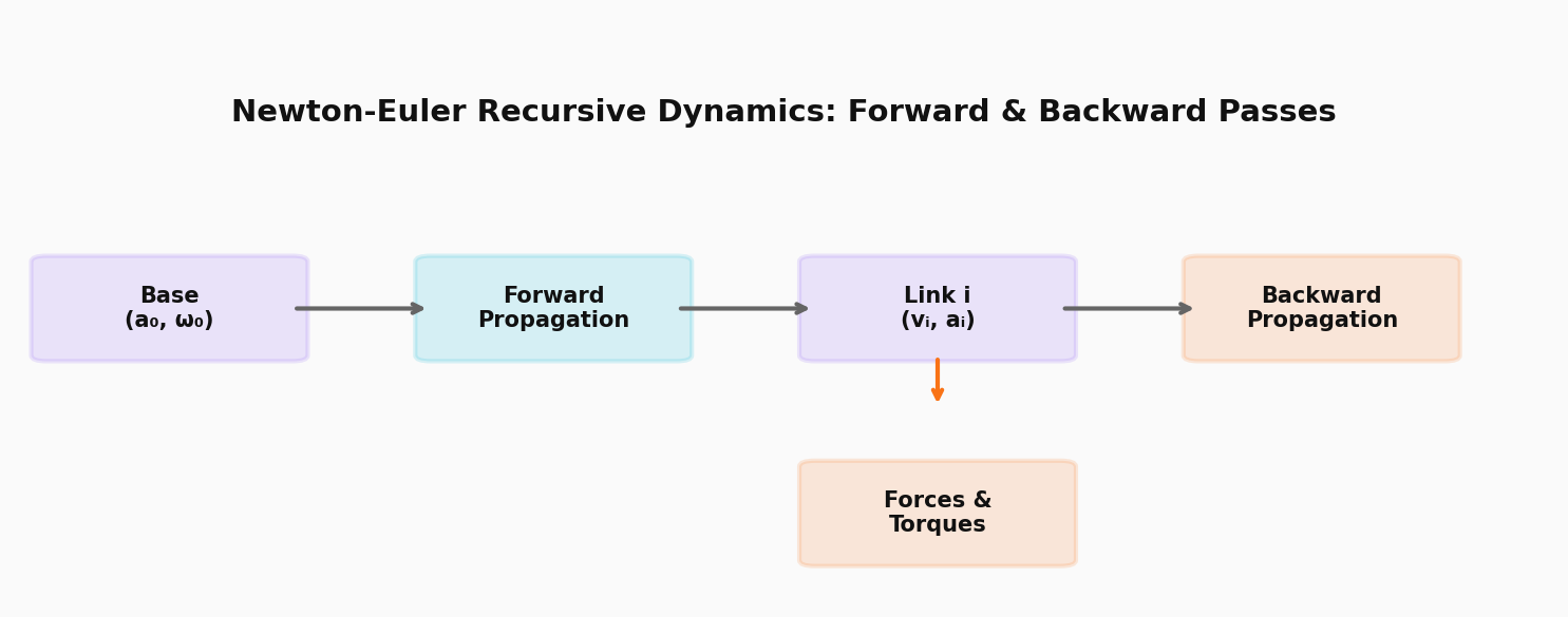
This mirrors how physical causality works: base motion propagates outward, while contact forces propagate inward.
Forward Pass: Velocity and Acceleration Propagation
For each link i from base to end-effector:
Rotational Joint
ωᵢ = ωᵢ₋₁ + q̇ᵢ · zᵢ
αᵢ = αᵢ₋₁ + q̈ᵢ · zᵢ + ωᵢ₋₁ × (q̇ᵢ · zᵢ)

aᵢ = aᵢ₋₁ + αᵢ × rᵢ + ωᵢ × (ωᵢ × rᵢ)
Where:
ω: Angular velocityα: Angular accelerationa: Linear acceleration of link framez: Joint axis (z-axis of joint frame)r: Vector from jointito linkiCOM
Prismatic Joint
ωᵢ = ωᵢ₋₁
αᵢ = αᵢ₋₁

aᵢ = aᵢ₋₁ + αᵢ × rᵢ + ωᵢ × (ωᵢ × rᵢ) + q̈ᵢ·zᵢ + 2·ωᵢ × (q̇ᵢ·zᵢ)
The 2·ω × (q̇·z) term is the Coriolis acceleration from sliding along a rotating link.
Backward Pass: Force and Torque Propagation
For each link i from end-effector to base:
import numpy as np

class RecursiveNewtonEuler:
    """
    Recursive Newton-Euler algorithm for serial chain robot dynamics
    """

    def __init__(self, links, joint_types):
        """
        Initialize robot parameters

        Args:
            links: List of link dicts with 'mass', 'com', 'inertia', 'axis', 'length'
            joint_types: List of 'revolute' or 'prismatic' for each joint
        """
        self.links = links
        self.joint_types = joint_types
        self.n = len(links)

    def skew_symmetric(self, w):
        """Create skew-symmetric matrix from vector w"""
        return np.array([
            [0, -w[2], w[1]],
            [w[2], 0, -w[0]],
            [-w[1], w[0], 0]
        ])

    def cross_product_matrix(self, w):
        """Alias for skew_symmetric"""
        return self.skew_symmetric(w)

    def forward_pass(self, q, dq, ddq, base_accel=None, base_omega=None):
        """
        Forward propagation of velocities and accelerations

        Args:
            q: Joint positions [n]
            dq: Joint velocities [n]
            ddq: Joint accelerations [n]
            base_accel: Base linear acceleration [3] (default: gravity)
            base_omega: Base angular velocity [3] (default: zero)

        Returns:
            velocities, accelerations for each link
        """
        if base_accel is None:
            base_accel = np.array([0, 0, -9.81])  # Gravity
        if base_omega is None:
            base_omega = np.zeros(3)

        # Initialize
        omega = [np.zeros(3) for _ in range(self.n)]
        alpha = [np.zeros(3) for _ in range(self.n)]
        accel = [np.zeros(3) for _ in range(self.n)]

        # Base conditions
        omega_prev = base_omega.copy()
        alpha_prev = np.zeros(3)
        accel_prev = base_accel.copy()

        for i in range(self.n):
            link = self.links[i]
            z_axis = np.array(link['axis'])

            if self.joint_types[i] == 'revolute':
                # Angular velocity and acceleration
                omega[i] = omega_prev + dq[i] * z_axis
                alpha[i] = alpha_prev + ddq[i] * z_axis + np.cross(omega_prev, dq[i] * z_axis)

                # Linear acceleration of link frame
                r_i = np.array(link.get('r_i', [link['length'], 0, 0]))
                accel[i] = (accel_prev + np.cross(alpha[i], r_i) +
                           np.cross(omega[i], np.cross(omega[i], r_i)))

            else:  # prismatic
                omega[i] = omega_prev.copy()
                alpha[i] = alpha_prev.copy()

                r_i = np.array(link.get('r_i', [link['length'], 0, 0]))
                accel[i] = (accel_prev + np.cross(alpha[i], r_i) +
                           np.cross(omega[i], np.cross(omega[i], r_i)) +
                           ddq[i] * z_axis + 2 * np.cross(omega[i], dq[i] * z_axis))

            # Update for next iteration
            omega_prev = omega[i]
            alpha_prev = alpha[i]
            accel_prev = accel[i]

        return omega, alpha, accel

    def backward_pass(self, omega, alpha, accel, external_forces=None, external_torques=None):
        """
        Backward propagation of forces and torques

        Args:
            omega, alpha, accel: From forward pass
            external_forces: External force at each link COM [n, 3]
            external_torques: External torque at each link [n, 3]

        Returns:
            joint_forces, joint_torques
        """
        if external_forces is None:
            external_forces = [np.zeros(3) for _ in range(self.n)]
        if external_torques is None:
            external_torques = [np.zeros(3) for _ in range(self.n)]

        # Force and torque at each joint (from link i+1 acting on link i)
        f = [np.zeros(3) for _ in range(self.n + 1)]
        tau = [np.zeros(3) for _ in range(self.n + 1)]

        # End-effector wrench (default: zero)
        f[self.n] = np.zeros(3)
        tau[self.n] = np.zeros(3)

        joint_torques = np.zeros(self.n)

        for i in range(self.n - 1, -1, -1):
            link = self.links[i]
            m = link['mass']
            I = np.array(link['inertia'])
            r_com = np.array(link.get('r_com', [link['length']/2, 0, 0]))

            # COM acceleration
            a_com = accel[i] + np.cross(alpha[i], r_com) + np.cross(omega[i], np.cross(omega[i], r_com))

            # Force balance: f[i] - f[i+1] + m*g = m*a_com
            f[i] = f[i+1] + m * a_com - external_forces[i]

            # Torque balance about COM
            r_joint_to_com = r_com
            r_com_to_next_joint = np.array(link.get('r_next', [link['length'], 0, 0])) - r_com

            tau[i] = (tau[i+1] - np.cross(f[i], r_joint_to_com) +
                     np.cross(f[i+1], r_com_to_next_joint) +
                     I @ alpha[i] + np.cross(omega[i], I @ omega[i]) -
                     external_torques[i])

            # Extract joint torque (component along joint axis)
            z_axis = np.array(link['axis'])
            if self.joint_types[i] == 'revolute':
                joint_torques[i] = np.dot(tau[i], z_axis)
            else:
                joint_torques[i] = np.dot(f[i], z_axis)

        return joint_torques, f, tau

    def compute_dynamics(self, q, dq, ddq, base_accel=None, base_omega=None):
        """
        Complete recursive Newton-Euler computation

        Args:
            q, dq, ddq: Joint state
            base_accel: Base acceleration (default: gravity)
            base_omega: Base angular velocity

        Returns:
            joint_torques [n]
        """
        omega, alpha, accel = self.forward_pass(q, dq, ddq, base_accel, base_omega)
        joint_torques, _, _ = self.backward_pass(omega, alpha, accel)
        return joint_torques

# Example: 2-DOF planar arm
links = [
    {
        'mass': 1.0,
        'inertia': [[0, 0, 0], [0, 0, 0], [0, 0, 0.05]],
        'axis': [0, 0, 1],
        'length': 0.6,
        'r_com': [0.3, 0, 0],
        'r_next': [0.6, 0, 0]
    },
    {
        'mass': 0.8,
        'inertia': [[0, 0, 0], [0, 0, 0], [0, 0, 0.03]],
        'axis': [0, 0, 1],
        'length': 0.5,
        'r_com': [0.25, 0, 0],
        'r_next': [0.5, 0, 0]
    }
]

robot = RecursiveNewtonEuler(links, ['revolute', 'revolute'])

# Test: static pose with gravity
q = np.array([0.5, 1.0])
dq = np.array([0.0, 0.0])
ddq = np.array([0.0, 0.0])

tau = robot.compute_dynamics(q, dq, ddq)
print(f"Joint torques (static, gravity only):")
print(f"τ₁ = {tau[0]:.3f} N·m")
print(f"τ₂ = {tau[1]:.3f} N·m")

# Test: accelerating from rest
ddq = np.array([2.0, 1.0])
tau_accel = robot.compute_dynamics(q, dq, ddq)
print(f"\nJoint torques (q̈₁=2, q̈₂=1):")
print(f"τ₁ = {tau_accel[0]:.3f} N·m")
print(f"τ₂ = {tau_accel[1]:.3f} N·m")
Extracting the Mass Matrix Efficiently
The recursive algorithm can also extract the mass matrix in O(n) time per column:
def compute_mass_matrix_rne(robot, q):
    """
    Compute mass matrix using recursive Newton-Euler

    Method: M[:, j] = RNE(q, 0, e_j) - G(q)
    where e_j is unit vector in direction j
    """
    n = robot.n
    M = np.zeros((n, n))

    # Gravity vector
    zero_dq = np.zeros(n)
    zero_ddq = np.zeros(n)
    G = robot.compute_dynamics(q, zero_dq, zero_ddq)

    # Each column: unit acceleration in one joint, zero elsewhere
    for j in range(n):
        ddq = np.zeros(n)
        ddq[j] = 1.0

        tau_column = robot.compute_dynamics(q, zero_dq, ddq)
        M[:, j] = tau_column - G

    return M

# Verify against Lagrangian result
M_rne = compute_mass_matrix_rne(robot, q=np.array([0.5, 1.0]))
print("Mass matrix from Recursive N-E:")
print(M_rne)
Real-Time Control Integration
Here’s how the recursive algorithm fits into a control loop:
class RealTimeRobotController:
    """
    High-frequency robot controller using recursive Newton-Euler
    """

    def __init__(self, robot_model, control_freq=1000):
        self.robot = robot_model
        self.dt = 1.0 / control_freq
        self.target_q = None
        self.target_dq = None

        # PD gains
        self.Kp = np.array([100.0, 50.0])
        self.Kd = np.array([20.0, 10.0])

    def compute_control_torque(self, q, dq, t):
        """
        Compute torque at each control cycle

        Total time budget: ~1 ms at 1 kHz
        - RNE dynamics: ~0.05 ms
        - PD control: ~0.01 ms
        - Safety checks: ~0.02 ms
        - Communication: ~0.3 ms
        - Headroom: ~0.6 ms
        """
        if self.target_q is None:
            return np.zeros(self.robot.n)

        # Desired trajectory (simple interpolation)
        q_des = self.target_q
        dq_des = self.target_dq if self.target_dq is not None else np.zeros(self.robot.n)
        ddq_des = np.zeros(self.robot.n)

        # Feedforward: compute torques for desired motion
        tau_ff = self.robot.compute_dynamics(q_des, dq_des, ddq_des)

        # Feedback: PD correction
        q_err = q_des - q
        dq_err = dq_des - dq
        tau_fb = self.Kp * q_err + self.Kd * dq_err

        # Total torque
        tau_total = tau_ff + tau_fb

        # Safety: torque limits
        tau_max = np.array([50.0, 30.0])  # N·m
        tau_total = np.clip(tau_total, -tau_max, tau_max)

        return tau_total

    def control_loop(self, q_current, dq_current, t):
        """One iteration of the control loop"""
        tau = self.compute_control_torque(q_current, dq_current, t)

        # In reality: send tau to motor drivers
        # Read next sensor values
        # Repeat

        return tau

# Example usage
controller = RealTimeRobotController(robot, control_freq=1000)
controller.target_q = np.array([1.0, 0.5])
controller.target_dq = np.array([0.0, 0.0])

tau_cmd = controller.control_loop(
    q_current=np.array([0.8, 0.4]),
    dq_current=np.array([0.2, 0.1]),
    t=0.0
)
print(f"Control torque: τ₁={tau_cmd[0]:.2f}, τ₂={tau_cmd[1]:.2f}")
Computational Complexity Analysis
| Operation | Operations per link | Total (n links) |
|---|---|---|
| Forward pass | ~30 FLOPs | 30n |
| Backward pass | ~40 FLOPs | 40n |
| Total per evaluation | ~70n FLOPs |
For a 6-DOF robot: ~420 FLOPs → ~0.4 μs on a 1 GHz processor. For a 20-DOF humanoid: ~1400 FLOPs → ~1.4 μs.
This leaves enormous headroom for sensor fusion, trajectory generation, and communication.
Key Takeaways
- Recursive Newton-Euler runs in O(n) time, making it the algorithm of choice for real-time control
- Forward pass propagates velocities and accelerations from base to end-effector
- Backward pass propagates forces and torques from end-effector to base
- The algorithm naturally handles gravity, Coriolis, and external forces
- Mass matrix extraction is O(n²) but each column is O(n), making it practical for control
- Industrial robots (ABB, KUKA, FANUC) use variants of this algorithm at 1-8 kHz
Next Steps
Tomorrow, we’ll implement a complete Python dynamics simulation environment using our derived equations, and validate against ground-truth simulators like PyBullet and MuJoCo.
Practice Exercise: Extend the recursive algorithm to handle a robot with a payload at the end-effector. How does a 2 kg payload at the end-effector change the required joint torques compared to an unloaded robot? Plot τ₁ and τ₂ as functions of payload mass from 0 to 5 kg.
Disclaimer
For educational purposes only. This article is part of a structured learning curriculum and does not constitute professional engineering advice.