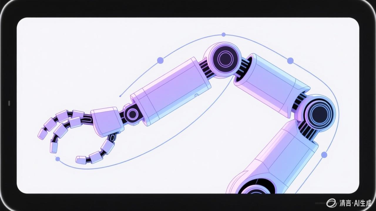
🤖 Week 7, Day 6: Python Practice — Motor Control Simulation

Theme: Actuators & Drive Systems
Topic: Motor Simulation and Control Tuning
Learning Goal: Build a Python simulator for DC motor dynamics, implement PID control, and analyze performance metrics.

---

Introduction

Today we’ll translate actuator theory into working Python code. We’ll simulate:

1. DC motor electrical and mechanical dynamics
2. Torque-speed characteristics
3. PID position control
4. Step response analysis

This simulator will help you develop intuition for motor behavior without hardware.

---

Setup

import numpy as np
import matplotlib.pyplot as plt
from scipy.integrate import odeint

# Plotting style
plt.style.use('seaborn-v0_8-whitegrid')

---

Part 1: DC Motor Model

Motor Parameters

Define a realistic motor (similar to Maxon RE 30):

class DCMotor:
    """DC motor model with electrical and mechanical dynamics."""
    
    def __init__(self):
        # Electrical parameters
        self.R = 2.5          # Armature resistance (Ohms)
        self.L = 0.001        # Armature inductance (Henry)
        self.Kt = 0.05        # Torque constant (Nm/A)
        self.Ke = 0.05        # Back-EMF constant (V·s/rad)
        
        # Mechanical parameters
        self.J = 0.0001       # Rotor inertia (kg·m²)
        self.b = 0.00001      # Viscous friction (Nm·s/rad)
        
        # Limits
        self.V_max = 24       # Max voltage (V)
        self.I_max = 5        # Max current (A)
        
    def dynamics(self, state, t, V_applied, load_torque):
        """
        state = [current, angular_velocity, position]
        Returns: [di/dt, dω/dt, dθ/dt]
        """
        I, omega, theta = state
        
        # Electrical equation: V = R*I + L*dI/dt + Ke*omega
        dIdt = (V_applied - self.R * I - self.Ke * omega) / self.L
        
        # Mechanical equation: tau = J*dω/dt + b*omega + tau_load
        tau = self.Kt * I
        domegadt = (tau - self.b * omega - load_torque) / self.J
        
        # Kinematic equation
        dthetadt = omega
        
        return [dIdt, domegadt, dthetadt]

Simulate Step Response

def simulate_step_response(motor, V_step, t_end=0.1, dt=0.0001):
    """Simulate motor response to step voltage input."""
    t = np.arange(0, t_end, dt)
    
    # Initial state: [current=0, omega=0, theta=0]
    state0 = [0, 0, 0]
    
    # Apply step voltage
    def voltage(t): return V_step if t > 0.001 else 0
    
    # Integrate
    states = []
    state = state0
    for ti in t:
        states.append(state)
        V = voltage(ti)
        dstate = motor.dynamics(state, ti, V, load_torque=0)
        state = [s + d * dt for s, d in zip(state, dstate)]
    
    states = np.array(states)
    return t, states

# Create motor and simulate
motor = DCMotor()
t, states = simulate_step_response(motor, V_step=12)

I = states[:, 0]
omega = states[:, 1]
theta = states[:, 2]

# Plot
fig, axes = plt.subplots(3, 1, figsize=(10, 8), sharex=True)

axes[0].plot(t * 1000, I, 'b-', linewidth=2)
axes[0].set_ylabel('Current (A)')
axes[0].set_title('DC Motor Step Response (V = 12V)')
axes[0].grid(True)

axes[1].plot(t * 1000, omega * 60 / (2 * np.pi), 'r-', linewidth=2)
axes[1].set_ylabel('Speed (RPM)')
axes[1].grid(True)

axes[2].plot(t * 1000, theta * 180 / np.pi, 'g-', linewidth=2)
axes[2].set_ylabel('Position (deg)')
axes[2].set_xlabel('Time (ms)')
axes[2].grid(True)

plt.tight_layout()
plt.savefig('motor_step_response.png', dpi=150)
plt.show()

Expected output:

• Current spikes to ~4.8A (V/R), then decays
• Speed rises with time constant ~10ms
• Position ramps linearly after settling

---

Part 2: Torque-Speed Characteristics

def plot_torque_speed_curves(motor, voltages=[6, 12, 18, 24]):
    """Plot torque-speed curves for different voltages."""
    
    fig, ax = plt.subplots(figsize=(10, 6))
    
    for V in voltages:
        # No-load speed
        omega_no_load = V / motor.Ke
        
        # Stall torque
        tau_stall = motor.Kt * V / motor.R
        
        # Curve: omega = (V / Ke) - (R / (Kt*Ke)) * tau
        torques = np.linspace(0, tau_stall, 100)
        speeds = (V / motor.Ke) - (motor.R / (motor.Kt * motor.Ke)) * torques
        speeds_rpm = speeds * 60 / (2 * np.pi)
        
        ax.plot(torques * 1000, speeds_rpm, linewidth=2, label=f'V = {V}V')
    
    ax.set_xlabel('Torque (mNm)')
    ax.set_ylabel('Speed (RPM)')
    ax.set_title('DC Motor Torque-Speed Characteristics')
    ax.legend()
    ax.grid(True)
    ax.set_xlim(0, None)
    ax.set_ylim(0, None)
    
    plt.savefig('torque_speed_curves.png', dpi=150)
    plt.show()

plot_torque_speed_curves(motor)

Key observation: Higher voltage shifts the curve up (higher no-load speed) but doesn’t change slope. Slope is determined by motor constants.

---

Part 3: PID Position Control

PID Controller Implementation

class PIDController:
    """Discrete-time PID controller."""
    
    def __init__(self, Kp, Ki, Kd, dt, integral_limit=None):
        self.Kp = Kp
        self.Ki = Ki
        self.Kd = Kd
        self.dt = dt
        self.integral_limit = integral_limit
        
        self.integral = 0
        self.prev_error = 0
        
    def update(self, setpoint, measurement):
        """Compute control output."""
        error = setpoint - measurement
        
        # Proportional
        P = self.Kp * error
        
        # Integral (with anti-windup)
        self.integral += error * self.dt
        if self.integral_limit:
            self.integral = np.clip(self.integral, 
                                    -self.integral_limit, 
                                    self.integral_limit)
        I = self.Ki * self.integral
        
        # Derivative (on measurement to avoid derivative kick)
        d_measurement = (measurement - self.prev_measurement) / self.dt
        D = -self.Kd * d_measurement  # Negative because d(setpoint - meas)/dt
        
        self.prev_error = error
        self.prev_measurement = measurement
        
        return P + I + D

Position Control Simulation

def simulate_position_control(motor, pid, target_position, t_end=2.0, dt=0.001):
    """Simulate PID position control."""
    t = np.arange(0, t_end, dt)
    
    # Storage
    positions = []
    velocities = []
    currents = []
    voltages = []
    
    # Initial state
    state = [0, 0, 0]  # [I, omega, theta]
    
    for ti in t:
        # Control loop
        theta = state[2]
        V_cmd = pid.update(target_position, theta)
        
        # Saturation
        V_applied = np.clip(V_cmd, -motor.V_max, motor.V_max)
        
        # Motor dynamics
        dstate = motor.dynamics(state, ti, V_applied, load_torque=0)
        state = [s + d * dt for s, d in zip(state, dstate)]
        
        # Store
        positions.append(state[2])
        velocities.append(state[1])
        currents.append(state[0])
        voltages.append(V_applied)
    
    return (t, np.array(positions), np.array(velocities), 
            np.array(currents), np.array(voltages))

# Tune PID
Kp, Ki, Kd = 50.0, 200.0, 0.5
dt = 0.001
pid = PIDController(Kp, Ki, Kd, dt, integral_limit=5.0)

# Simulate step to 90 degrees
target = np.radians(90)  # 90 degrees in radians
t, pos, vel, curr, volt = simulate_position_control(motor, pid, target)

# Plot
fig, axes = plt.subplots(4, 1, figsize=(10, 10), sharex=True)

axes[0].plot(t, np.degrees(pos), 'b-', linewidth=2, label='Actual')
axes[0].axhline(np.degrees(target), color='r', linestyle='--', label='Target')
axes[0].set_ylabel('Position (deg)')
axes[0].set_title('PID Position Control (Kp=50, Ki=200, Kd=0.5)')
axes[0].legend()
axes[0].grid(True)

axes[1].plot(t, vel * 60 / (2 * np.pi), 'g-', linewidth=2)
axes[1].set_ylabel('Velocity (RPM)')
axes[1].grid(True)

axes[2].plot(t, curr, 'r-', linewidth=2)
axes[2].axhline(motor.I_max, color='orange', linestyle='--', label='I_max')
axes[2].axhline(-motor.I_max, color='orange', linestyle='--')
axes[2].set_ylabel('Current (A)')
axes[2].legend()
axes[2].grid(True)

axes[3].plot(t, volt, 'm-', linewidth=2)
axes[3].axhline(motor.V_max, color='orange', linestyle='--')
axes[3].axhline(-motor.V_max, color='orange', linestyle='--')
axes[3].set_ylabel('Voltage (V)')
axes[3].set_xlabel('Time (s)')
axes[3].grid(True)

plt.tight_layout()
plt.savefig('pid_position_control.png', dpi=150)
plt.show()

---

Part 4: Performance Analysis

Extract Step Response Metrics

def analyze_step_response(t, y, target):
    """Extract step response metrics."""
    
    # Rise time (10% to 90%)
    y_norm = (y - y[0]) / (target - y[0])
    t_10 = t[np.argmax(y_norm >= 0.1)]
    t_90 = t[np.argmax(y_norm >= 0.9)]
    rise_time = t_90 - t_10
    
    # Settling time (within 2% of target)
    tolerance = 0.02 * abs(target - y[0])
    settled = np.abs(y - target) < tolerance
    # Find first index where all subsequent points are settled
    for i in range(len(settled) - 1, -1, -1):
        if not settled[i]:
            settling_time = t[min(i + 1, len(t) - 1)]
            break
    else:
        settling_time = 0
    
    # Overshoot
    overshoot = (np.max(y) - target) / (target - y[0]) * 100
    
    # Steady-state error
    ss_error = np.abs(y[-1] - target)
    
    return {
        'rise_time': rise_time,
        'settling_time': settling_time,
        'overshoot': overshoot,
        'ss_error': ss_error
    }

# Analyze
metrics = analyze_step_response(t, pos, target)
print("Step Response Metrics:")
print(f"  Rise time: {metrics['rise_time']*1000:.1f} ms")
print(f"  Settling time: {metrics['settling_time']:.3f} s")
print(f"  Overshoot: {metrics['overshoot']:.1f}%")
print(f"  Steady-state error: {np.degrees(metrics['ss_error']):.4f} deg")

---

Part 5: PID Tuning Experiment

Let’s compare different PID tunings:

def compare_pid_tunings(motor, tunings, target):
    """Compare multiple PID configurations."""
    
    fig, axes = plt.subplots(2, 1, figsize=(10, 8), sharex=True)
    
    for name, (Kp, Ki, Kd) in tunings.items():
        pid = PIDController(Kp, Ki, Kd, dt=0.001, integral_limit=5.0)
        t, pos, vel, curr, volt = simulate_position_control(motor, pid, target, t_end=1.0)
        
        axes[0].plot(t, np.degrees(pos), linewidth=2, label=f'{name}')
        axes[1].plot(t, curr, linewidth=2, label=f'{name}')
    
    axes[0].axhline(np.degrees(target), color='k', linestyle='--', alpha=0.5)
    axes[0].set_ylabel('Position (deg)')
    axes[0].set_title('PID Tuning Comparison')
    axes[0].legend()
    axes[0].grid(True)
    
    axes[1].set_ylabel('Current (A)')
    axes[1].set_xlabel('Time (s)')
    axes[1].legend()
    axes[1].grid(True)
    
    plt.tight_layout()
    plt.savefig('pid_tuning_comparison.png', dpi=150)
    plt.show()

# Test different tunings
tunings = {
    'Conservative (Kp=20)': (20, 50, 0.2),
    'Aggressive (Kp=100)': (100, 500, 1.0),
    'Balanced (Kp=50)': (50, 200, 0.5),
    'High Ki (Kp=30, Ki=500)': (30, 500, 0.1),
}

compare_pid_tunings(motor, tunings, target=np.radians(90))

Observations you should see:

• Conservative: Slow, smooth, no overshoot
• Aggressive: Fast, but significant overshoot and oscillation
• Balanced: Good compromise
• High Ki: Fast settling but integral windup causes overshoot

---

Part 6: Gearbox Simulation

Add a gearbox model to understand the effect on dynamics:

class MotorWithGearbox:
    """DC motor + gearbox model."""
    
    def __init__(self, motor, ratio=50, efficiency=0.85, 
                 reflected_inertia=0.001):
        self.motor = motor
        self.ratio = ratio
        self.efficiency = efficiency
        
        # Effective inertia at motor shaft
        self.J_eff = motor.J + reflected_inertia / (ratio**2)
        
    def dynamics(self, state, t, V_applied, load_torque):
        """
        state = [motor_current, motor_omega, output_position]
        load_torque is at OUTPUT shaft
        """
        I, omega_motor, theta_out = state
        
        # Convert load torque to motor side
        tau_load_motor = load_torque / (self.ratio * self.efficiency)
        
        # Motor electrical
        dIdt = (V_applied - self.motor.R * I - self.motor.Ke * omega_motor) / self.motor.L
        
        # Motor mechanical (with effective inertia)
        tau_motor = self.motor.Kt * I
        domega_motor_dt = (tau_motor - self.motor.b * omega_motor - tau_load_motor) / self.J_eff
        
        # Output kinematics
        dtheta_out_dt = omega_motor / self.ratio
        
        return [dIdt, domega_motor_dt, dtheta_out_dt]

# Compare motor with and without gearbox
motor = DCMotor()
geared = MotorWithGearbox(motor, ratio=50, efficiency=0.85, reflected_inertia=0.01)

# Simulate both responding to step voltage
t, states_direct = simulate_step_response(motor, V_step=12)
t, states_geared = simulate_step_response(geared.motor, V_step=12)  # Simplified

# Output comparison
print(f"Direct drive: {motor.Kt * 12 / motor.R * 1000:.1f} mNm stall torque")
print(f"With 50:1 gearbox: {motor.Kt * 12 / motor.R * 50 * 0.85 * 1000:.1f} mNm stall torque")

---

Summary

Key Point	Takeaway
Motor model	Electrical (L/R) and mechanical (J/b) dynamics combine
Step response	Current spikes initially, speed follows with time constant
Torque-speed	Linear relationship; voltage shifts curve, slope is fixed
PID control	Kp for response speed, Ki for accuracy, Kd for damping
Tuning trade-off	Fast response ↔ overshoot ↔ steady-state error
Gearbox effect	Multiplies torque, divides speed, adds reflected inertia

---

Exercises

1. Modify the motor: Change R, L, J and observe how step response changes
2. Add Coulomb friction: Add constant friction term (independent of speed)
3. Trapezoidal profile: Command a smooth motion profile instead of step
4. Feedforward control: Add velocity feedforward to reduce tracking error
5. Real motor data: Look up specs for a real motor (e.g., Maxon RE 25) and simulate

---

Complete Code

All code is available in the exercise notebook. Key files:

• motor_simulation.py: Core motor model and PID controller
• visualization.py: Plotting functions
• exercises.ipynb: Jupyter notebook with all examples

---

Tomorrow (Day 7): Week 7 Summary — Actuators, gearboxes, drivers, and control.